← Data and chance

Data and chance: recap

Answer each question in your head or on paper first, then check it.

Data

1. Counting and measuring

Try firstClassify: (a) number of apps on a phone, (b) battery temperature, (c) screen size in inches. Explain one.

Check your answer

(a) discrete (counted), (b) continuous (measured), (c) continuous (measured, though sold in common sizes).

Discrete data is counted: it takes separate values, such as 0, 1, 2 siblings. Continuous data is measured: it can be any value in a range, such as a 100 m time of 14.37 s.

Measured values are always rounded: 152 cm to the nearest centimetre means from 151.5 cm up to 152.5 cm. Decimals alone do not make data continuous: shoe sizes (7, 7.5, 8) are discrete.
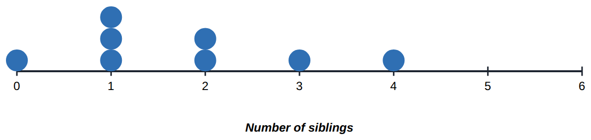
Number of siblings: counted, so only whole numbers (discrete). Nobody has 1.5 siblings.
Counted or measured? · Sound on for the voiceover
Open the lesson →

2. Mean, median, mode and range

Try firstFind the mean, median, mode and range of 6, 2, 9, 6, 7, 12.

Check your answer

Mean 42 ÷ 6 = 7; median (6 + 7) ÷ 2 = 6.5; mode 6; range 10.

Four numbers sum up a data set:

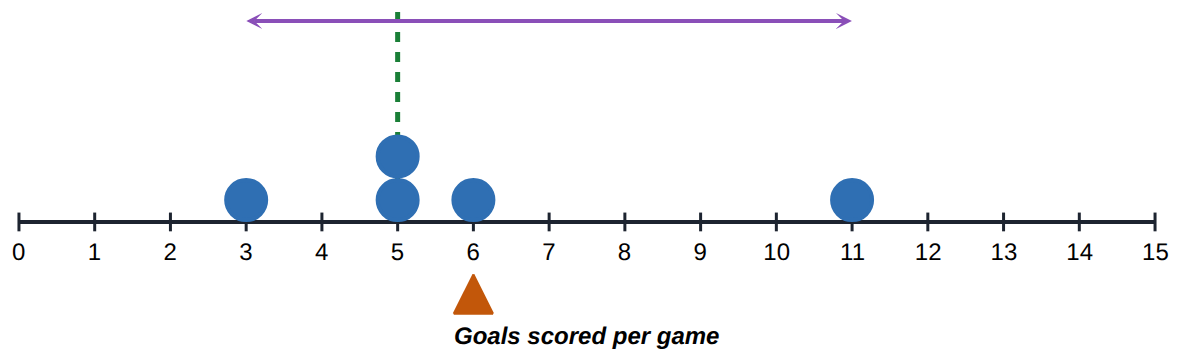
  • mean: add the values, then divide by how many there are (3, 5, 5, 6, 11: 30 ÷ 5 = 6);
  • median: sort the values and take the middle one; for an even count, halfway between the two middle values;
  • mode: the most common value (there can be two, or none);
  • range: highest minus lowest (11 − 3 = 8), a measure of spread.
3, 5, 5, 6, 11: mean 6 (▲), median 5 (dashed), mode 5, range 11 − 3 = 8 (arrow).
Four numbers that sum up the data · Sound on for the voiceover
Open the lesson →

3. Which measure?

Try firstSalaries in a small company ($ thousands): 50, 52, 55, 58, 400. Which measure would you report as typical, and why?

Check your answer

The median, 55: the 400 is an outlier that pulls the mean up to 123, more than four of the five salaries.

The mean, median and mode can disagree. Look for outliers first (values far from the rest):

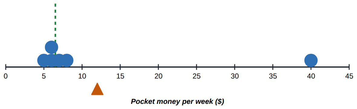
  • An outlier pulls the mean towards it, so with one the median usually describes a typical value better ($5, 6, 6, 7, 8, 40$: mean 12, median 6.5).
  • With no outliers, the mean is a fair summary because it uses every value.
  • For "which is most common?", use the mode.
One outlier (40) pulls the mean (▲) up to 12, past every other value; the median (dashed) stays at 6.5, among the typical values.
An outlier drags the mean · Sound on for the voiceover
Open the lesson →

4. Stem-and-leaf plots

Try firstDraw a stem-and-leaf plot of 17, 25, 22, 41, 18, 29, 26 and find its median.

Check your answer

1 | 7 8, 2 | 2 5 6 9, 3 | (empty), 4 | 1. Median: the 4th of 7 values, 25.

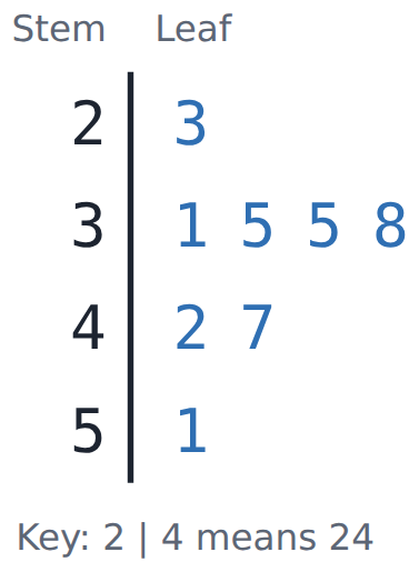
A stem-and-leaf plot keeps every value and shows the shape. For two-digit numbers the stem is the tens digit and the leaf is the units digit; leaves go in order along their stem's row. Include every stem from the smallest to the largest, even with no leaves, and give a key: $3 \mid 5$ means $35$.

Read the median by counting leaves to the middle; the range is the last value minus the first.

Stems are the tens, leaves the units, in order: 3 | 1 5 5 8 is 31, 35, 35 and 38.
Tens as stems, units as leaves · Sound on for the voiceover
Open the lesson →

5. Comparing data sets

Try firstGroup 1 reaction times (s): median 0.32, range 0.10. Group 2: median 0.28, range 0.35. Compare the groups in one sentence.

Check your answer

Group 2 was faster on a typical try (median 0.28 s against 0.32 s), but much less consistent (range 0.35 s against 0.10 s).

Describe a data set by its shape (symmetrical, or skewed with a tail; clusters, gaps, outliers), its centre (median or mean) and its spread (range).

To compare two sets, compare the centres and the spreads, with numbers and in context: "Similar medians (15 and 16), but Class A is more consistent (range 6 against 16)." One value, such as the highest score, does not describe a set.

Class B's median (16) is a little higher, but its range (16) is much wider than Class A's (6): A is more consistent.
Compare centre and spread · Sound on for the voiceover
Open the lesson →

9. Statistical investigations

Try firstA survey asks only the first 10 students into school how they travel. Give one reason it may not represent the school.

Check your answer

Students who arrive early may travel differently (for example, by bus or parent drop-off), so the sample is biased.

A statistical investigation asks a question data can answer, plans the variable and a fair sample, collects and displays the data, summarises its shape, centre and spread, and reports an answer with its limits.

A sample that is small or chosen for convenience may be biased, so the report says who was measured and how.

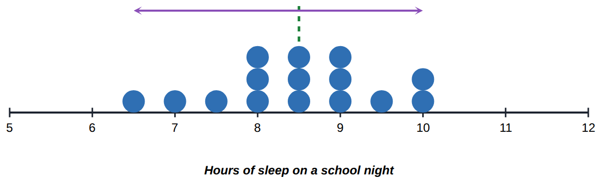
Fifteen students' hours of sleep: the median is 8.5 hours and the range is 3.5 hours.
From a question to a report · Sound on for the voiceover
Open the lesson →

Chance

6. Sample spaces and probability

Try firstA bag has 2 red, 3 green and 5 yellow counters. List the sample space and give each probability.

Check your answer

{red, green, yellow}: P(red) = 2/10 = 1/5, P(green) = 3/10, P(yellow) = 5/10 = 1/2. They add to 1.

The sample space is the list of every possible outcome. If the outcomes are equally likely,

$P(\text{event}) = \dfrac{\text{favourable outcomes}}{\text{total outcomes}}$, so $P(\text{even on a dice}) = \tfrac{3}{6} = \tfrac{1}{2}$.

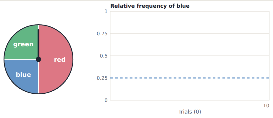
If they are not (a half-red spinner, a bag with more of one colour), use the sizes or the counts: $P(\text{red}) = \tfrac{1}{2}$. The probabilities of all the outcomes add to 1; 0 means impossible, 1 means certain.

Sample space {red, blue, green}, but not equally likely: P(red) = 1/2, P(blue) = 1/4, P(green) = 1/4. They add to 1.
List the outcomes, then share out the chance · Sound on for the voiceover
Open the lesson →

7. Predict and test

Try firstA spinner has P(blue) = 0.4. How many blues do you expect in 50 spins? You get 23. Is the spinner unfair?

Check your answer

20 expected. 23 is close to 20, so there is no reason to think it is unfair.

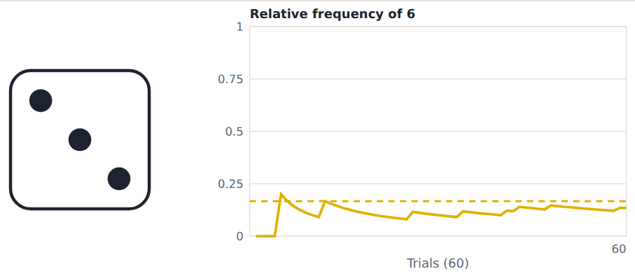
A probability predicts what happens over many trials: expected count = probability × number of trials. In 60 rolls of a fair dice, expect about $60 \times \tfrac{1}{6} = 10$ sixes.

Then test it: run the experiment and record the counts. The relative frequency is count ÷ trials. In a short experiment the results vary: 7 or 12 sixes in 60 rolls is normal, so do not judge a dice on a few rolls.

60 rolls: about 10 sixes expected (60 × 1/6). The actual count is near 10, but not exactly 10.
Expected count, then the real count · Sound on for the voiceover
Open the lesson →

8. Many trials

Try firstAfter 40 spins a spinner gave 18 reds; after 4000 spins, 1230 reds. Which estimate of P(red) is better, and what is it?

Check your answer

The 4000-spin one: 1230 ÷ 4000 ≈ 0.31. More trials give a more reliable estimate.

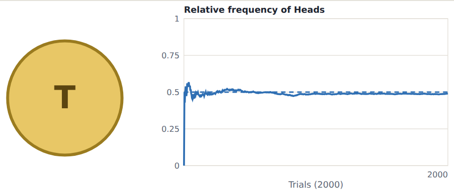
Over a few trials, the relative frequency (count ÷ trials) jumps about. Over many trials it settles close to the probability: the law of large numbers. One more head moves 7/10 a lot, but 501/1000 hardly at all.

It is not because results balance out: a coin has no memory, and after 5 tails heads is still exactly 1/2. Large experiments are how we estimate probabilities we cannot work out, such as a drawing pin landing point-up.

2000 flips: the relative frequency of heads jumps about at first, then settles near 0.5 (dashed).
More trials, a steadier estimate · Sound on for the voiceover
Open the lesson →

10. Complementary events

Try firstP(it snows tomorrow) = 0.08. What is P(it does not snow)? Then: two coins are tossed; what is P(at least one tail)?

Check your answer

0.92. And 1 − P(HH) = 1 − 1/4 = 3/4.

The complement of an event A, written not A, is every other outcome. A and not A cover every outcome exactly once, so P(A) + P(not A) = 1, and P(not A) = 1 − P(A).

This makes at least one easy: count the outcomes with none, and subtract from 1. Two events that just can't happen together are not complementary unless they cover every outcome too.

A dice: A is 'roll 1 or 2' (blue, 2 outcomes); not A is the other 4 (orange). 2/6 + 4/6 = 1.
An event and its complement · Sound on for the voiceover
Open the lesson →

11. Venn diagrams and two-way tables

Try first50 students: 30 study French, 25 study Japanese, 10 study both. How many study neither?

Check your answer

French only 20, Japanese only 15, both 10: 45, so 5 study neither.

Sorting a group by two yes/no properties makes four groups: one only, the other only, both and neither. Everyone is in exactly one.

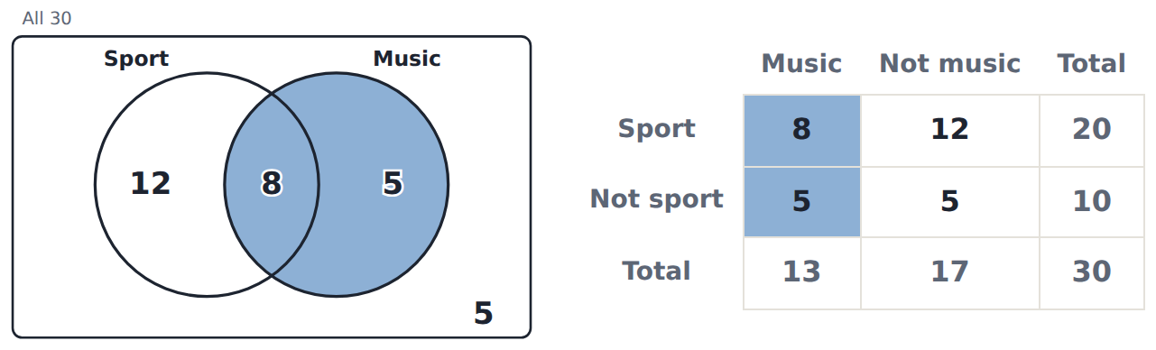
A Venn diagram shows them as two overlapping circles in a box; a two-way table shows them as four cells with totals. Write both first, then take it from each total.

30 students: 12 sport only, 8 both, 5 music only, 5 neither. Music (shaded) is 8 + 5 = 13: the table's Music total.
Four groups, two pictures · Sound on for the voiceover
Open the lesson →

12. Grids and tree diagrams

Try firstA spinner shows 1, 2 or 3 (equal parts) and a coin is tossed. List the outcomes. What is P(an odd number and heads)?

Check your answer

1H, 1T, 2H, 2T, 3H, 3T: 6 outcomes. 1H and 3H, so 2/6 = 1/3.

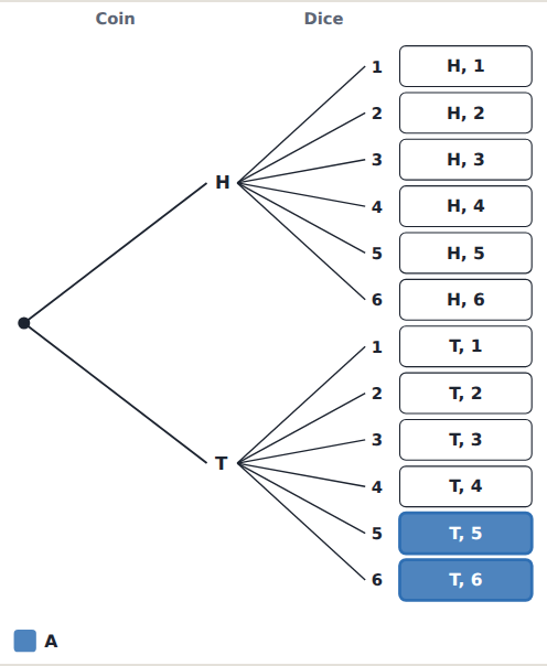
Two events one after the other make pairs. A tree diagram splits each first outcome into every second outcome; a grid puts one event down the side and the other across. Both list every pair once, so each is equally likely.

The number of outcomes is the two counts multiplied. Order matters: HT and TH are different outcomes. Then P(event) = outcomes in the event ÷ all outcomes.

A coin then a dice: 2 branches, then 6 from each, makes 12 outcomes. Tails and more than 4: 2 of them.
A tree diagram · Sound on for the voiceover
Open the lesson →

13. And, or and not

Try first40 students: 25 like maths, 18 like art, 10 like both. Find P(maths or art) and P(neither).

Check your answer

25 + 18 − 10 = 33, so 33/40. Neither: 7/40.

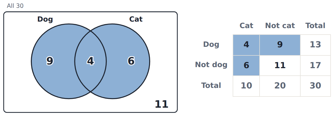
A and B: both happen (the overlap). A or B: at least one happens, both included (everything inside the circles). Not A: everything outside A. Neither: outside both.

Count each outcome once. From totals: P(A or B) = P(A) + P(B) − P(A and B), because the overlap is in both totals.

Dog or cat: everything inside the circles, 9 + 4 + 6 = 19. The 4 with both are counted once.
And, or · Sound on for the voiceover
Open the lesson →

14. Simulating compound events

Try firstA simulation gives a total of 8 on two dice 68 times in 500 trials. Find the relative frequency and compare it with the probability.

Check your answer

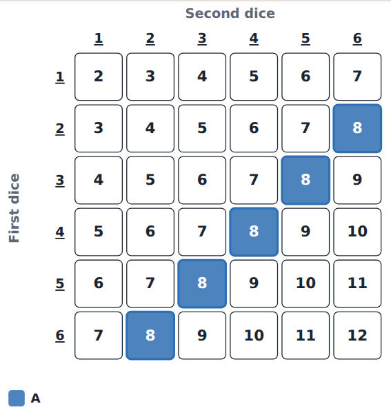
68 ÷ 500 = 0.136. P(8) = 5/36 ≈ 0.139: very close.

A simulation repeats a chance experiment many times with random numbers. Record each result in a frequency table, then relative frequency = count ÷ trials.

Compare it with the probability from the sample space. A short run can be well off; over many trials the relative frequency settles close to the probability. A simulation estimates; the grid gives the exact value.

Two dice: a total of 8 is 5 of the 36 outcomes, P = 5/36 ≈ 0.14. A simulation's relative frequency should come close to this over many trials.
A simulation · Sound on for the voiceover
Open the lesson →

Samples

15. Census, sample, experiment or observation

Try firstA cereal company wants to check the weight of its boxes. Census or sample? Why?

Check your answer

A sample: weighing every box costs time; checking a random sample of boxes each hour is enough to spot problems.

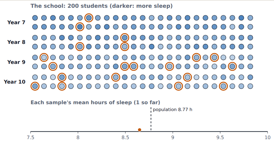
The population is everyone the question is about. A census measures all of them (exact, but often slow and costly); a sample measures some (quicker and cheaper, an estimate).

An experiment changes something on purpose and measures the effect; an observation watches without changing anything. Choose the technique that fits the question, the cost and the time.

The population: 200 students in four year groups. A census measures all of them; this random sample (orange rings) measures 20.
Census or sample · Sound on for the voiceover
Open the lesson →

16. Bias in collecting data

Try firstA gym surveys its members on how often people exercise. Name the bias and which way it pushes the result.

Check your answer

Sampling bias: gym members exercise more than most people, so the result is too high.

Bias is anything in how data is collected that pushes the result one way. Sampling bias: the sample isn't like the population (only people at a gym). Response bias: the question or setting pushes answers (leading questions, no privacy). Measurement bias: the tool or method is off.

A bigger sample doesn't fix bias. Random choice, neutral questions, anonymous answers and checked tools do.

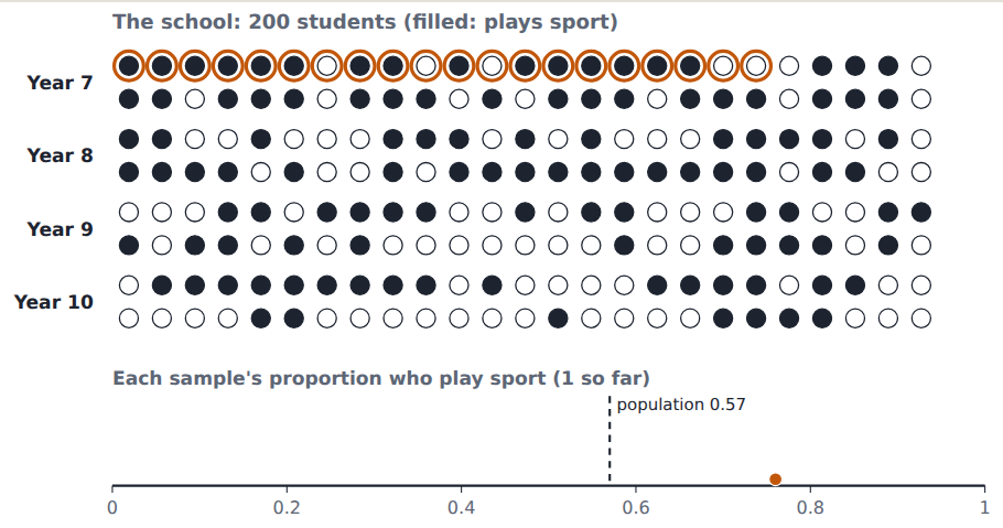
A convenience sample: the 20 students nearest the door, all from Year 7. Year 7s play more sport, so the sample overstates the school's proportion.
A biased sample · Sound on for the voiceover
Open the lesson →

17. Ways to choose a sample

Try firstA school has 400 Year 9 and 200 Year 10 students. Describe how to take a stratified sample of 30.

Check your answer

In proportion: 20 Year 9s and 10 Year 10s, each chosen at random from its year's list.

Simple random: every member has the same chance. Systematic: every kth member of a list from a random start (k = population ÷ sample size). Stratified: split into groups and choose at random within each, in proportion, so each group gets its fair share. Convenience: whoever is easiest, often biased. Quota: fixed shares, but the collector chooses, so it can be biased too.

A stratified sample of 20: 5 chosen at random from each year group, so every year has its fair share.
Four ways to choose · Sound on for the voiceover
Open the lesson →

18. Describing a sample

Try firstA random sample of 25 students spends a median of 40 minutes on homework a night (range 0 to 120). Write one sentence about the school.

Check your answer

Students at the school probably spend about 40 minutes on homework a night, though some spend much more, based on a random sample of 25.

To report on a sample: describe its shape (symmetric or skewed, clusters, outliers), centre (mean, median) and spread (range). Then give an estimate for the population, with the sampling method and size, using words like "about".

Primary data you collect yourself; secondary data someone else collected. Either way, say where it came from.

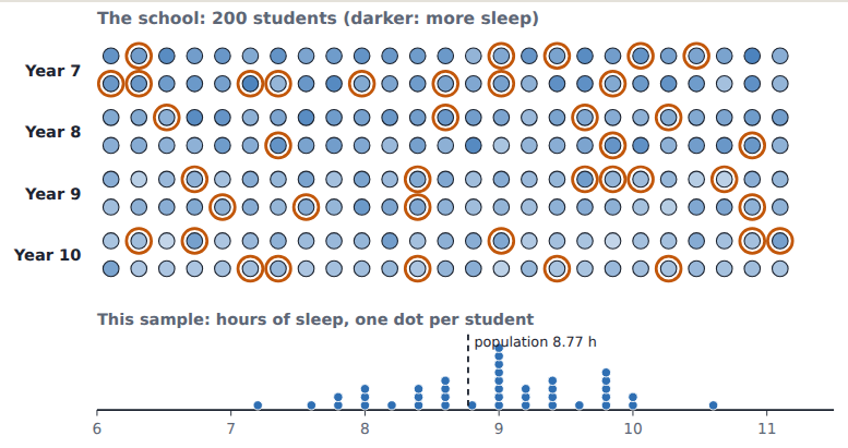
A random sample of 40 students' sleep: most between 8 and 10 hours, a few lower. The dashed line is the whole school's mean.
Reporting on a sample · Sound on for the voiceover
Open the lesson →

19. How samples vary

Try firstTwo random samples of 10 students give 0.4 and 0.7 for the proportion who walk to school. Is one wrong? What would you do?

Check your answer

Not necessarily: small samples vary a lot. Take bigger samples (or more of them) for a more reliable estimate.

Sampling variation: random samples from the same population give different results, because each holds different members. It isn't a mistake.

Bigger samples vary less, so their results are more reliable. Fair samples scatter around the population's value; bias pushes them all to one side.

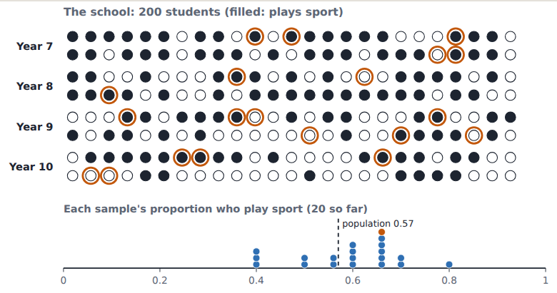
20 random samples of 20 students: each gives a different proportion who play sport, scattered around the school's 0.57 (dashed).
Samples vary · Sound on for the voiceover
Open the lesson →

20. Investigating with samples

Try firstA random sample of 50 students at your school shows a median of 2 hours of screen time on school nights. Write an inference with its uncertainty.

Check your answer

Students at our school probably have about 2 hours of screen time on school nights, from a random sample of 50; another sample might give a slightly different value.

An investigation with samples asks a question about a population, plans a fair and ethical sample (random, consent, anonymous, neutral questions), collects and describes the data, then makes an inference.

A good inference is about the population sampled, gives an estimate ("about"), and states the uncertainty: the sample's size and method, and that another sample might differ a little.

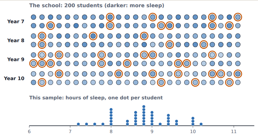
A random sample of 40 with the population hidden: the sample's centre is the estimate, and the population's value is unknown.
Inferring from a sample · Sound on for the voiceover
Open the lesson →