← Data and chance

Maths reference: Data and chance

The words and methods from Data and chance, each with an example and, where it helps, a picture of the board.

Print a cheat sheet (the whole course or one unit, with board pictures)

Data

counted: discretemeasured: continuous\text{counted: discrete} \quad \text{measured: continuous}
discrete and continuous

Discrete data takes separate values (number of siblings). Continuous data can be any value in a range (height, time), and is rounded when recorded.

mean=totalnumber of values=305=6\text{mean} = \dfrac{\text{total}}{\text{number of values}} = \dfrac{30}{5} = 6
mean

Add the values, then share equally. An outlier pulls the mean towards it.
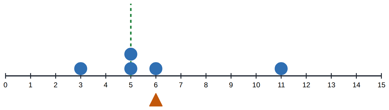
3, 5, 5, 6, 11: mean 6 (▲), median 5 (dashed)
3,4,6,7‾,8,9→6+72=6.53, 4, \underline{6, 7}, 8, 9 \to \tfrac{6 + 7}{2} = 6.5
median

Sort first; the middle value, or halfway between the two middle values for an even count.

mode: most commonrange=highest−lowest\text{mode: most common} \quad \text{range} = \text{highest} - \text{lowest}
mode and range

There can be two modes, or none. The range is a simple measure of spread.

5,6,6,7,8,40: median 6.55, 6, 6, 7, 8, \mathbf{40}:\ \text{median } 6.5
choosing a measure

With an outlier, the median describes a typical value better than the mean. Without, the mean uses every value. For 'most common', use the mode.

3∣1 5 5 8=31,35,35,383 \mid 1\ 5\ 5\ 8 = 31, 35, 35, 38
stem-and-leaf plot

Tens as stems, units as leaves in order; include every stem, even with no leaves; give a key.

Stems are the tens, leaves the units
centre (15,16) and spread (6,16)\text{centre } (15, 16) \text{ and spread } (6, 16)
comparing data sets

Describe shape (symmetrical or skewed, clusters, gaps, outliers), centre and spread. Compare both centre and spread, with numbers, in context.

Similar medians; Class B much more spread
ask→plan→collect→display→summarise→report\text{ask} \to \text{plan} \to \text{collect} \to \text{display} \to \text{summarise} \to \text{report}
statistical investigation

Ask a question data can answer, plan the variable and a fair sample, collect and display the data, describe its shape, centre and spread, then report the answer with its limits.

Chance

{1,2,3,4,5,6}\{1, 2, 3, 4, 5, 6\}
sample space

Every possible outcome, listed once. Check whether the outcomes are equally likely.

P(even)=favourabletotal=36=12P(\text{even}) = \dfrac{\text{favourable}}{\text{total}} = \dfrac{3}{6} = \dfrac{1}{2}
probability

For equally likely outcomes. Otherwise use sizes or counts. From 0 (impossible) to 1 (certain); all outcomes add to 1.
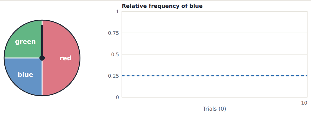
A half-red spinner: P(red) = 1/2, P(blue) = P(green) = 1/4
60×16=1060 \times \tfrac{1}{6} = 10
expected count

Expected count = probability × trials. Real results vary around it, more so in short experiments.

counttrials=1320=0.65\dfrac{\text{count}}{\text{trials}} = \dfrac{13}{20} = 0.65
relative frequency

The experiment's estimate of the probability. Over many trials it settles close to the probability (the law of large numbers); nothing is ever 'due'.
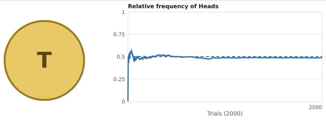
2000 flips: the relative frequency of heads settles near 0.5
P(not A)=1−P(A)P(\text{not } A) = 1 - P(A)
complementary events

An event and its complement cover every outcome once. For 'at least one', count the outcomes with none and subtract from 1.
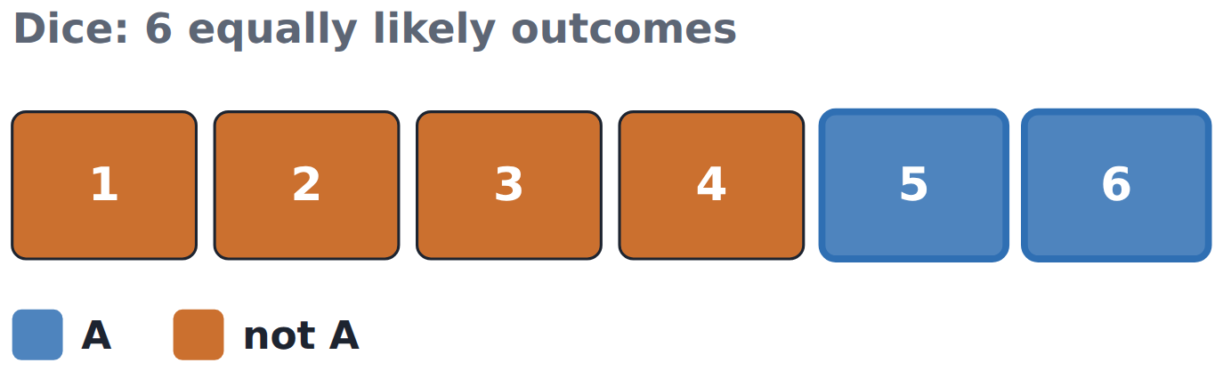
Roll 5 or 6 (A) and the other four outcomes (not A)
both first: only=total−both\text{both first: only} = \text{total} - \text{both}
Venn diagram and two-way table

Two yes/no properties make four groups: one only, both, the other only, neither. Each is a region of the Venn diagram and a cell of the table.
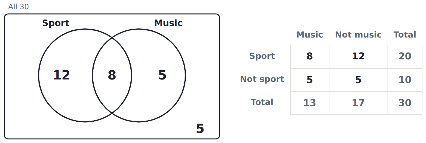
The same 30 students as a Venn diagram and a two-way table
outcomes=3×2=6\text{outcomes} = 3 \times 2 = 6
grid and tree diagram

Two events make pairs: a grid or a tree lists every pair once, and the number of outcomes is the two counts multiplied. HT and TH are different outcomes.
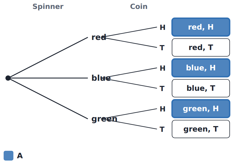
A spinner with three equal parts, then a coin: 6 outcomes, 3 of them heads
P(A or B)=P(A)+P(B)−P(A and B)P(A \text{ or } B) = P(A) + P(B) - P(A \text{ and } B)
and, or, not

And is the overlap; or is one, the other or both; not A is everything outside A. Count each outcome once.
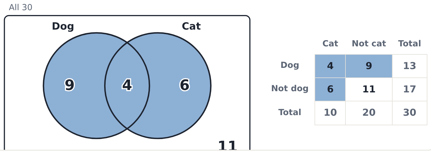
Dog or cat: everything inside the circles, 19 of 30
relative frequency=counttrials\text{relative frequency} = \dfrac{\text{count}}{\text{trials}}
simulation

Run many trials with random numbers (=RANDBETWEEN(1,6) is a dice) and compare the relative frequency with the probability. Short runs can be well off.

Two dice with a total of 10 or more chosen (6 of 36), ready to simulate

Samples

census: everyonesample: some\text{census: everyone} \quad \text{sample: some}
census and sample

A census is exact but slow and costly; a sample estimates. An experiment changes something on purpose; an observation watches.

A random sample of 20 from a school of 200
who? how asked? how measured?\text{who? how asked? how measured?}
bias

Bias pushes a result one way: sampling bias (who is asked), response bias (how they are asked), measurement bias (the tool). A bigger sample doesn't fix it.
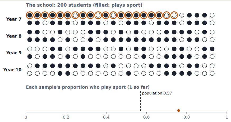
A convenience sample: all from Year 7, pushed high
k=populationsample sizek = \dfrac{\text{population}}{\text{sample size}}
sampling methods

Simple random: same chance for all. Systematic: every kth from a random start. Stratified: at random within each group, in proportion. Convenience and quota: someone chooses, so they can be biased.

shape, centre, spread→about …\text{shape, centre, spread} \to \text{about } \ldots
describing a sample

Describe the shape (symmetric or skewed), the centre (mean, median) and the spread (range), then estimate the population with the method and size. Primary data you collect; secondary data others collected.
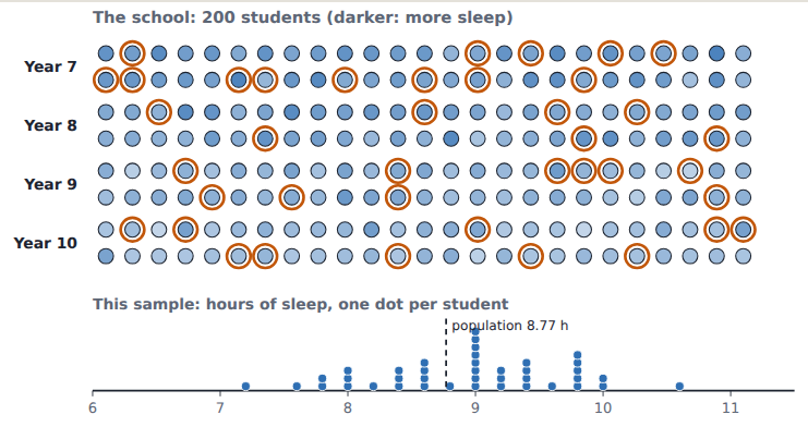
A random sample of 40 students' sleep as a dot plot
bigger samples vary less\text{bigger samples vary less}
sampling variation

Fair samples from one population give different results by chance. Their results scatter around the population's value, closer for bigger samples.

20 samples of 20: results scattered around the school's value
about …, from a random sample of n\text{about } \ldots \text{, from a random sample of } n
inference

Infer only about the population sampled, give an estimate, and say how sure you are (size and method). Collect data with consent and anonymity.