← Reference

Data and chance: cheat sheet

Data and chance · The words and methods from the lessons, with an example of each.

Data

discrete and continuous

Discrete data takes separate values (number of siblings). Continuous data can be any value in a range (height, time), and is rounded when recorded.

counted: discretemeasured: continuous\text{counted: discrete} \quad \text{measured: continuous}

median

Sort first; the middle value, or halfway between the two middle values for an even count.

3,4,6,7‾,8,9→6+72=6.53, 4, \underline{6, 7}, 8, 9 \to \tfrac{6 + 7}{2} = 6.5

mode and range

There can be two modes, or none. The range is a simple measure of spread.

mode: most commonrange=highest−lowest\text{mode: most common} \quad \text{range} = \text{highest} - \text{lowest}

stem-and-leaf plot

Tens as stems, units as leaves in order; include every stem, even with no leaves; give a key.

3∣1 5 5 8=31,35,35,383 \mid 1\ 5\ 5\ 8 = 31, 35, 35, 38
Stems are the tens, leaves the units

statistical investigation

Ask a question data can answer, plan the variable and a fair sample, collect and display the data, describe its shape, centre and spread, then report the answer with its limits.

ask→plan→collect→display→summarise→report\text{ask} \to \text{plan} \to \text{collect} \to \text{display} \to \text{summarise} \to \text{report}

mean

Add the values, then share equally. An outlier pulls the mean towards it.
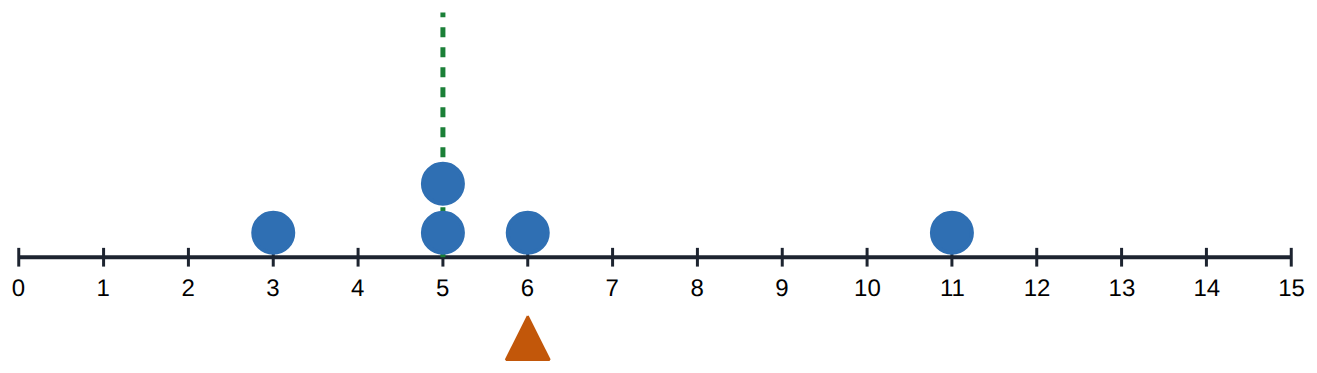
mean=totalnumber of values=305=6\text{mean} = \dfrac{\text{total}}{\text{number of values}} = \dfrac{30}{5} = 6
3, 5, 5, 6, 11: mean 6 (▲), median 5 (dashed)

choosing a measure

With an outlier, the median describes a typical value better than the mean. Without, the mean uses every value. For 'most common', use the mode.

5,6,6,7,8,40: median 6.55, 6, 6, 7, 8, \mathbf{40}:\ \text{median } 6.5

comparing data sets

Describe shape (symmetrical or skewed, clusters, gaps, outliers), centre and spread. Compare both centre and spread, with numbers, in context.

centre (15,16) and spread (6,16)\text{centre } (15, 16) \text{ and spread } (6, 16)
Similar medians; Class B much more spread

Chance

sample space

Every possible outcome, listed once. Check whether the outcomes are equally likely.

{1,2,3,4,5,6}\{1, 2, 3, 4, 5, 6\}

expected count

Expected count = probability × trials. Real results vary around it, more so in short experiments.

60×16=1060 \times \tfrac{1}{6} = 10

relative frequency

The experiment's estimate of the probability. Over many trials it settles close to the probability (the law of large numbers); nothing is ever 'due'.
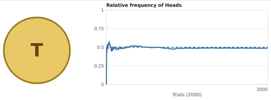
counttrials=1320=0.65\dfrac{\text{count}}{\text{trials}} = \dfrac{13}{20} = 0.65
2000 flips: the relative frequency of heads settles near 0.5

Venn diagram and two-way table

Two yes/no properties make four groups: one only, both, the other only, neither. Each is a region of the Venn diagram and a cell of the table.
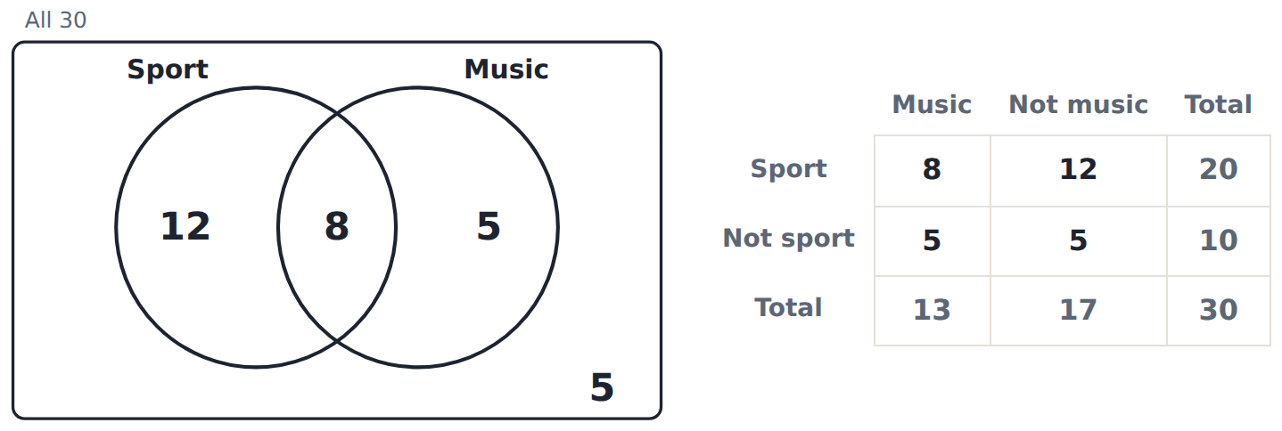
both first: only=total−both\text{both first: only} = \text{total} - \text{both}
The same 30 students as a Venn diagram and a two-way table

and, or, not

And is the overlap; or is one, the other or both; not A is everything outside A. Count each outcome once.
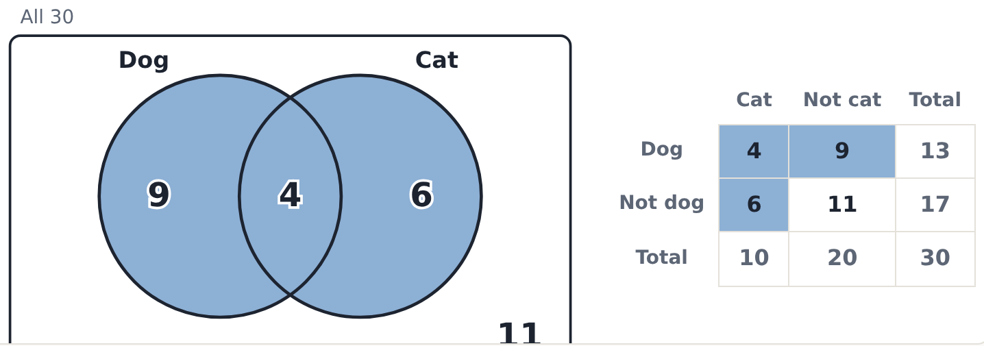
P(A or B)=P(A)+P(B)−P(A and B)P(A \text{ or } B) = P(A) + P(B) - P(A \text{ and } B)
Dog or cat: everything inside the circles, 19 of 30

probability

For equally likely outcomes. Otherwise use sizes or counts. From 0 (impossible) to 1 (certain); all outcomes add to 1.
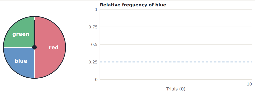
P(even)=favourabletotal=36=12P(\text{even}) = \dfrac{\text{favourable}}{\text{total}} = \dfrac{3}{6} = \dfrac{1}{2}
A half-red spinner: P(red) = 1/2, P(blue) = P(green) = 1/4

complementary events

An event and its complement cover every outcome once. For 'at least one', count the outcomes with none and subtract from 1.
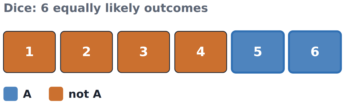
P(not A)=1−P(A)P(\text{not } A) = 1 - P(A)
Roll 5 or 6 (A) and the other four outcomes (not A)

grid and tree diagram

Two events make pairs: a grid or a tree lists every pair once, and the number of outcomes is the two counts multiplied. HT and TH are different outcomes.
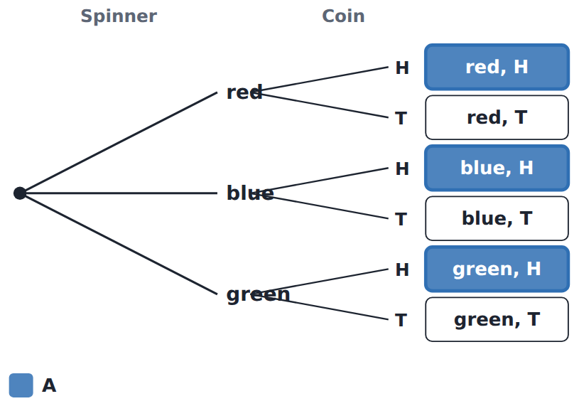
outcomes=3×2=6\text{outcomes} = 3 \times 2 = 6
A spinner with three equal parts, then a coin: 6 outcomes, 3 of them heads

simulation

Run many trials with random numbers (=RANDBETWEEN(1,6) is a dice) and compare the relative frequency with the probability. Short runs can be well off.

relative frequency=counttrials\text{relative frequency} = \dfrac{\text{count}}{\text{trials}}
Two dice with a total of 10 or more chosen (6 of 36), ready to simulate

Samples

census and sample

A census is exact but slow and costly; a sample estimates. An experiment changes something on purpose; an observation watches.

census: everyonesample: some\text{census: everyone} \quad \text{sample: some}
A random sample of 20 from a school of 200

sampling methods

Simple random: same chance for all. Systematic: every kth from a random start. Stratified: at random within each group, in proportion. Convenience and quota: someone chooses, so they can be biased.

k=populationsample sizek = \dfrac{\text{population}}{\text{sample size}}

sampling variation

Fair samples from one population give different results by chance. Their results scatter around the population's value, closer for bigger samples.

bigger samples vary less\text{bigger samples vary less}
20 samples of 20: results scattered around the school's value

bias

Bias pushes a result one way: sampling bias (who is asked), response bias (how they are asked), measurement bias (the tool). A bigger sample doesn't fix it.
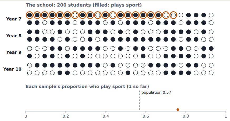
who? how asked? how measured?\text{who? how asked? how measured?}
A convenience sample: all from Year 7, pushed high

describing a sample

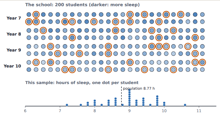
Describe the shape (symmetric or skewed), the centre (mean, median) and the spread (range), then estimate the population with the method and size. Primary data you collect; secondary data others collected.
shape, centre, spread→about …\text{shape, centre, spread} \to \text{about } \ldots
A random sample of 40 students' sleep as a dot plot

inference

Infer only about the population sampled, give an estimate, and say how sure you are (size and method). Collect data with consent and anonymity.

about …, from a random sample of n\text{about } \ldots \text{, from a random sample of } n